Time series annotation is the process of adding structured labels anomaly markers, event boundaries, pattern classifications, and state tags to sequential data that changes over time, so that machine learning models can learn to detect events, predict failures, and classify temporal patterns in sensor streams, physiological signals, and IoT telemetry.

This is one of the most underserved annotation disciplines in the industry. While image and text annotation have thousands of dedicated guides, tools, and service providers, time series annotation operates in the background of some of the most critical AI applications: cardiac monitoring systems that detect arrhythmias, factory equipment that predicts its own failures, and power grids that identify faults before they cascade.

Sensor data annotation encompasses a range of tasks from simple binary labeling (“normal” vs. “anomalous”) to complex multi-channel waveform annotation across EEG, ECG, and EMG signals. What makes time series data labeling distinct from other annotation types is that annotators work with continuous, often noisy signals where patterns unfold over time not with discrete images, documents, or text snippets. The annotator must understand temporal context: a spike that is normal at 2 PM during machine startup may be an anomaly at 2 AM during idle operation.

The demand for time series annotation is growing rapidly as IoT deployments scale across manufacturing, healthcare, energy, transportation, and smart infrastructure. An estimated 41.6 billion IoT devices will be in operation by 2025 (IDC), each generating continuous data streams that require annotated training data to power AI-driven monitoring, prediction, and automation.

This guide covers every major method in time series annotation, from anomaly marking to physiological waveform annotation, with the specificity that sensor AI teams need.

Anomaly Detection Labeling: Marking What Should Not Be There

Anomaly detection labeling is the process of identifying and tagging unusual patterns, outliers, or deviations in time-series data that differ from expected normal behavior. It is the most common form of time series annotation and the foundation of predictive maintenance, fraud detection, healthcare monitoring, and infrastructure security systems.

How it works

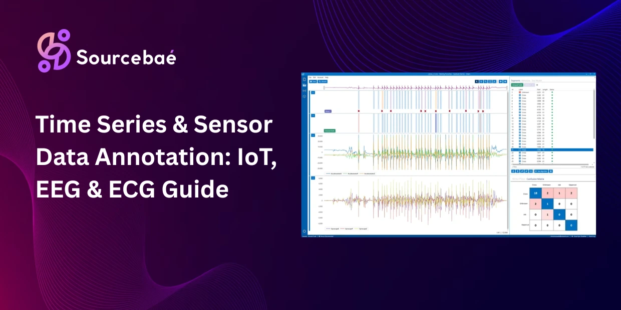
Annotators review continuous time-series signals and mark the time windows where anomalous behavior occurs. Each anomaly is tagged with a start timestamp, end timestamp, and typically a class label (equipment failure, sensor malfunction, security breach, cardiac arrhythmia, etc.). Some schemas also include severity ratings minor anomaly, major anomaly, critical event.

Anomaly detection labeling is inherently challenging because anomalies are rare. In most real-world datasets, anomalous events constitute less than 1–5% of the total data. This extreme class imbalance means that annotators spend the vast majority of their time confirming “normal” data and must maintain vigilance to catch the rare, brief events that matter most.

Use cases

Anomaly detection labeling powers cardiac arrhythmia detection from ECG signals, industrial equipment fault detection from vibration and temperature sensors, network intrusion detection from traffic flow data, financial fraud detection from transaction patterns, and power grid fault detection from voltage and frequency measurements.

Common pitfalls

Contextual anomalies are the primary annotation challenge. A reading of 95°C on a machine sensor is anomalous during normal operation but perfectly normal during a known heat-treatment cycle. Annotators need access to operational context shift schedules, maintenance logs, process phases not just the raw signal. Without this context, anomaly detection labeling produces labels that teach models to flag legitimate operational states as faults.

Annotation fatigue from class imbalance degrades quality. After hours of reviewing normal data, annotators begin to lose focus precisely when an anomaly appears. Effective workflows use pre-screening tools that flag candidate anomalies for human review rather than requiring annotators to watch continuous streams.

Event Tagging and Temporal Segmentation

Event tagging annotation marks the start and end boundaries of specific events within a time-series stream and assigns each event a label from a predefined taxonomy. Unlike anomaly detection labeling, which focuses on deviations from normal, event tagging labels all significant occurrences both expected and unexpected.

How it works

Annotators review the time-series signal and place boundary markers where events begin and end. Each segmented event receives a class label: “machine startup,” “cutting cycle,” “cooldown phase,” “operator intervention,” “material change,” or any other event relevant to the domain. The output is a timeline of labeled events that transforms a continuous stream into a structured sequence the model can learn from.

Time series data labeling for events requires precise temporal boundary placement. In industrial applications, the difference between a “startup” event ending at timestamp 14:03:22 versus 14:03:45 can affect whether the model correctly learns the transition between operational phases.

Use cases

Manufacturing process phase detection (identifying each step in an assembly sequence), sports performance analysis (segmenting sprints, recovery periods, and technique phases), sleep stage classification (labeling REM, NREM stages from EEG), medical procedure phase recognition, and energy consumption pattern segmentation.

Common pitfalls

Gradual transitions make boundary placement ambiguous. When does “machine warmup” end and “steady-state operation” begin? The transition may span minutes, and two annotators may place the boundary at different points. Clear quantitative rules “startup ends when temperature stabilizes within ±2°C for 30 seconds” reduce boundary ambiguity.

Waveform Annotation for Physiological Signals: EEG, ECG, and EMG

Waveform annotation labels specific patterns, morphological features, and clinical events within physiological signals the rhythmic, oscillating data produced by the brain (EEG), heart (ECG), and muscles (EMG). This is the most specialized form of time series annotation, requiring annotators with clinical or neuroscience training to identify medically significant patterns that generalist labelers would miss.

EEG Annotation: Labeling Brain Activity

EEG annotation labels patterns in electroencephalogram recordings the electrical signals produced by the brain, captured through electrodes on the scalp. Annotators identify specific waveform morphologies: sleep spindles, K-complexes, spike-and-wave discharges (associated with epilepsy), alpha/beta/theta/delta rhythms, and artifacts caused by eye blinks or muscle movement.

EEG annotation is performed across multiple channels simultaneously a standard clinical EEG uses 19–21 electrodes, and high-density research setups may use 128–256 channels. Annotators must interpret patterns that emerge across channel combinations, not just individual channels, making EEG annotation one of the most cognitively demanding annotation tasks in any domain.

Use cases include epilepsy seizure detection and classification, sleep stage scoring (labeling REM, N1, N2, N3 stages per 30-second epochs), brain-computer interface training, anesthesia depth monitoring, and neurological disorder research (Parkinson’s, Alzheimer’s).

ECG Annotation: Labeling Cardiac Rhythms

ECG annotation labels the characteristic waveform features and rhythm patterns in electrocardiogram recordings. Annotators identify the P wave, QRS complex, T wave, and their intervals (PR, QT, RR) in each heartbeat cycle. They also classify rhythm abnormalities: atrial fibrillation, ventricular tachycardia, premature ventricular contractions, ST-segment elevation (indicating possible myocardial infarction), and bradycardia/tachycardia.

The MIT-BIH Arrhythmia Database remains the most widely used benchmark for ECG annotation research, containing 48 half-hour recordings with cardiologist-verified annotations. Modern wearable ECG devices sample at approximately 250 Hz, producing continuous data streams that require annotation for both model training and real-time monitoring system validation.

ECG annotation demands clinical expertise a misidentified arrhythmia in training data can teach a cardiac monitoring model to miss life-threatening events or generate dangerous false alarms. TinyML-based ECG classification systems deployed on edge devices have achieved approximately 97% accuracy on benchmark datasets, but this accuracy depends entirely on the quality of the underlying annotations.

EMG Annotation: Labeling Muscle Activity

EMG (electromyography) waveform annotation labels muscle activation patterns, contraction timing, fatigue signatures, and neuromuscular abnormalities. Annotators mark the onset and offset of muscle contractions, classify contraction types (voluntary, involuntary, spasm), and identify pathological patterns. EMG annotation powers prosthetic control systems, physical rehabilitation monitoring, ergonomic assessment tools, and neuromuscular disease diagnostics.

Common pitfalls across waveform annotation

Artifact contamination is the biggest challenge in physiological waveform annotation. Eye blinks contaminate EEG. Muscle movement corrupts ECG. Electrode displacement creates spurious patterns in all modalities. Annotators must distinguish genuine physiological events from artifacts a skill that requires clinical training, not just pattern recognition.

Multi-channel complexity multiplies annotation difficulty. A single EEG annotation task may involve reviewing 19+ channels simultaneously, identifying patterns that appear across specific channel combinations. This cannot be reduced to single-channel annotation without losing critical spatial information about brain activity.

IoT Data Annotation: Labeling Connected Device Streams

IoT data annotation labels the continuous data streams generated by networks of connected sensors temperature, pressure, vibration, humidity, flow rate, voltage, and hundreds of other measurements produced by industrial equipment, smart buildings, vehicles, and environmental monitoring systems.

How it works

IoT data annotation typically involves multivariate time series multiple sensor channels measured simultaneously from the same system. An industrial motor might generate vibration, temperature, current draw, and acoustic emission data simultaneously. Annotators must interpret patterns across these correlated channels, identifying events that manifest as coordinated changes across multiple sensors rather than anomalies in any single channel.

Graph Neural Networks (GNNs) are increasingly used to model inter-sensor dependencies in IoT data annotation workflows, learning which sensors are spatially or functionally related and using those relationships to improve anomaly detection.

Use cases

Smart building energy management (labeling HVAC cycles, occupancy patterns, efficiency anomalies), connected vehicle fleet monitoring (identifying driving behavior patterns, mechanical stress events), supply chain cold-chain monitoring (flagging temperature excursions in pharmaceutical shipments), agricultural sensor networks (labeling irrigation events, soil moisture anomalies), and smart city infrastructure monitoring (traffic flow patterns, utility consumption anomalies).

Common pitfalls

Sensor drift is a pervasive challenge in IoT data annotation. Sensors gradually lose calibration over time, producing readings that slowly shift from true values. A temperature sensor drifting 0.5°C per month may not trigger an anomaly threshold on any single day, but the cumulative drift corrupts the dataset over time. Annotators must distinguish genuine environmental changes from sensor drift a distinction that requires understanding both the sensor physics and the operational context.

Variable sampling rates across sensors complicate annotation. One sensor may report every second while another reports every minute. Aligning and annotating data across different temporal resolutions requires interpolation or resampling, each of which introduces assumptions that can affect annotation accuracy.

Predictive Maintenance Annotation: Labeling the Path to Failure

Predictive maintenance annotation is a specialized form of sensor data annotation that labels the degradation patterns leading up to equipment failure. Instead of marking individual anomalies, annotators label the progressive deterioration sequence the days or weeks of gradually worsening vibration, increasing temperature, or declining efficiency that precede a breakdown.

How it works

Annotators are given historical sensor data from equipment that eventually failed, along with maintenance records documenting when and how the failure occurred. Working backward from the failure event, they label the degradation phases: “normal operation,” “early degradation,” “accelerated degradation,” and “imminent failure.” This produces the training data for Remaining Useful Life (RUL) estimation models AI systems that predict how much operating time equipment has left before failure.

Use cases

Manufacturing equipment life prediction, aircraft engine health monitoring, wind turbine gearbox degradation tracking, railway infrastructure monitoring, and oil and gas pipeline integrity assessment.

Common pitfalls

Hindsight bias affects annotation quality. When annotators know that a failure occurred, they tend to “see” degradation signs earlier than they actually became detectable, creating labels that overestimate the model’s ability to predict failure in advance. Blind annotation protocols where annotators do not know whether the data leads to a failure help control this bias.

Key Challenges in Time-Series Annotation

Time series annotation faces challenges that other annotation domains do not encounter.

Noise and signal quality variability. Real-world sensor data is noisy. Electromagnetic interference, mechanical vibration, sensor aging, and environmental conditions all introduce noise that obscures the patterns annotators need to identify. Preprocessing filtering, denoising, normalization must be applied carefully before annotation, but over-filtering can remove genuine anomalies along with the noise.

Concept drift. The statistical properties of time-series data change over time. A manufacturing process optimized in January may produce different sensor signatures by June after tool wear, material changes, or environmental shifts. Models trained on January annotations may fail on June data. Time series data labeling must be treated as a continuous process, not a one-time batch.

Extreme class imbalance. Anomalies are rare by definition. In healthcare monitoring, a dangerous arrhythmia may appear in 0.1% of recorded heartbeats. In industrial monitoring, a critical fault may occur once per year. Training models on such imbalanced data requires careful annotation strategies oversampling anomalies, undersampling normal data, or using focal loss functions all of which depend on the accuracy and completeness of the original anomaly detection labeling.

Temporal resolution sensitivity. The same event looks different at different sampling rates. A vibration spike lasting 50 milliseconds is clearly visible at 1,000 Hz sampling but invisible at 1 Hz. Sensor data annotation guidelines must specify the temporal resolution at which annotations should be applied, and annotators must work at appropriate zoom levels.

Choosing the Right Time-Series Annotation Method

Choose anomaly detection labeling when your model must identify deviations from normal behavior equipment faults, cardiac arrhythmias, network intrusions, or financial fraud. This is the most common starting point for time series annotation projects.

Choose event tagging when your model must identify and classify specific occurrences process phases, sleep stages, activity transitions, or operational events. Time series data labeling for events requires precise temporal boundaries and clear event taxonomy design.

Choose waveform annotation when your model must interpret physiological signals EEG annotation for brain activity, ECG annotation for cardiac rhythms, or EMG annotation for muscle patterns. These tasks require domain-expert annotators with clinical training.

Choose IoT data annotation when your model must interpret multivariate sensor streams from connected devices factory equipment, smart buildings, vehicles, or environmental networks. IoT data annotation requires understanding inter-sensor relationships and operational context.

Choose predictive maintenance annotation when your model must estimate remaining equipment life by identifying progressive degradation patterns in historical sensor data.

Frequently Asked Questions

What is time series annotation?

Time series annotation is the process of labeling sequential data that changes over time. This includes sensor readings, physiological signals, financial data, and IoT telemetry. Annotators apply structured markers such as anomaly tags, event boundaries, pattern classifications, and state labels. Unlike image or text annotation, time series annotation requires temporal context. The meaning of a data point depends on what came before and after it. It powers anomaly detection, predictive maintenance, healthcare monitoring, and industrial AI applications.

What is sensor data annotation?

Sensor data annotation labels continuous data streams from physical sensors temperature, pressure, vibration, voltage, flow rate, and physiological measurements. It encompasses labeling for anomaly detection, event segmentation, predictive maintenance, and multivariate pattern classification. Sensor data annotation is distinct because it involves noisy, high-frequency data from multiple correlated channels, requiring annotators who understand both the sensor physics and the operational context.

What is anomaly detection labeling?

Anomaly detection labeling identifies and tags unusual patterns or deviations in time-series data that differ from expected normal behavior. Annotators mark anomalous time windows with start/end timestamps and class labels (equipment fault, arrhythmia, intrusion, fraud). The primary challenge is extreme class imbalance: anomalies typically constitute less than 1–5% of the data, meaning annotators spend most of their time confirming normal behavior and must maintain vigilance for rare events. Contextual anomalies events that are only abnormal in specific operational conditions require access to operational metadata beyond the raw signal.

What is EEG annotation?

EEG annotation labels specific patterns in electroencephalogram recordings of brain electrical activity. Annotators identify waveform morphologies like sleep spindles, spike-and-wave discharges (epilepsy markers), and frequency band rhythms across 19–256 simultaneous electrode channels. EEG annotation requires neuroscience or clinical training because patterns emerge across channel combinations, not individual channels. Primary applications include epilepsy seizure detection, sleep stage scoring, brain-computer interface training, and neurological disorder research.

What is ECG annotation?

ECG annotation labels waveform features and rhythm patterns in electrocardiogram recordings. Annotators identify the P wave, QRS complex, T wave, intervals (PR, QT, RR), and classify rhythm abnormalities such as atrial fibrillation, ventricular tachycardia, and ST-segment elevation. ECG annotation demands clinical expertise misidentified arrhythmias in training data can cause monitoring systems to miss life-threatening events. The MIT-BIH Arrhythmia Database (48 cardiologist-verified recordings) remains the benchmark for ECG research.

What is IoT data annotation?

IoT data annotation labels the continuous, multivariate data streams generated by networks of connected sensors. Unlike single-channel annotation, it involves interpreting patterns across correlated sensor channels. These include coordinated changes in vibration, temperature, and current draw that signal an emerging equipment fault. Key challenges include sensor drift from gradual calibration loss and variable sampling rates across sensors. Annotators also need operational context to distinguish genuine anomalies from expected process variations.

How much does time series data labeling cost?

Costs for time series data labeling vary dramatically by domain and complexity. Basic anomaly detection labeling on single-channel industrial data costs approximately $5–$15 per hour of recorded data. Multi-channel IoT data annotation costs $10–$30 per hour due to multivariate complexity. Clinical waveform annotation is the most expensive category. EEG annotation requiring neurologist review costs $50–$150+ per hour of recording. ECG annotation with cardiologist verification costs $30–$80 per hour. These costs reflect the domain expertise required. Clinical annotators command premium rates because their label accuracy directly impacts patient safety.

What tools are used for waveform annotation?

Specialized tools for waveform annotation include EDFbrowser and Persyst for clinical EEG review. Physionet’s annotation tools handle ECG data and integrate with the MIT-BIH database. Label Studio is an open-source option that supports time-series with custom annotation interfaces. Custom Grafana-based dashboards serve industrial IoT sensor visualization and annotation. For IoT data annotation, AWS Timestream and InfluxDB provide time-series storage. Both can pair with custom annotation interfaces for labeling workflows. Most general-purpose annotation platforms lack native time-series support. This makes domain-specific tooling essential for time series annotation projects.